Economie du travail

Définitions et faits stylisés

Les mesures du chômage

Au sens du BIT
Au sens de France Travail

Insee: L’essentiel sur le chômage

Le marché du travail

Offre de travail

Emane des salariés

Demande de travail

Emane des employeurs

L’arbitrage consommation-Loisirs

La contrainte budgétaire

Show the code

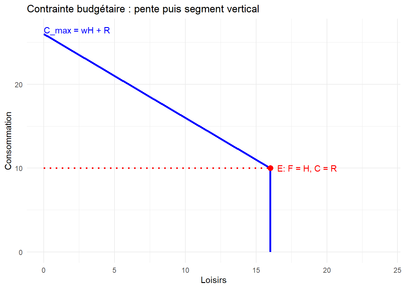
library(ggplot2)

# Paramètres
H <- 16
w <- 1
R <- 10
F_max <- 24

# Domaine pour la pente
F_vals <- seq(0, H, length.out = 300)
C_vals <- w*H + R - w*F_vals  # pente -w

df_pente <- data.frame(F = F_vals, C = C_vals)

# Point E
F_E <- H
C_E <- R  # = w*H + R - w*H

# C intercept (F = 0)
C_max <- w*H + R

# Tracé
ggplot() +
  # Droite de la contrainte (pente -w)
  geom_line(data = df_pente, aes(x = F, y = C), color = "blue", size = 1.2) +
  # Segment vertical bleu de E jusqu'à l'axe horizontal (C=0)
  geom_segment(aes(x = F_E, xend = F_E, y = 0, yend = C_E), color = "blue", size = 1.2) +
  # Segment horizontal pointillé rouge de E jusqu'à l'axe vertical (F=0, C=R)
  geom_segment(aes(x = 0, xend = F_E, y = C_E, yend = C_E), color = "red", linetype = "dotted", size = 1) +
  # Point E
  geom_point(aes(x = F_E, y = C_E), color = "red", size = 3) +
  # Annotation pour point E
  annotate("text", x = F_E + 0.5, y = C_E, label = paste0("E: F = H, C = R"), color = "red", hjust = 0) +
  # Annotation pour C intercept
  annotate("text", x = 0, y = C_max + 0.5, label = paste0("C_max = wH + R "), color = "blue", hjust = 0) +
  # Optionnel : un petit segment pour marquer C_max
  geom_segment(aes(x = -0.5, xend = 0, y = C_max, yend = C_max), color = "blue", size = 1) +
  labs(
    title = "Contrainte budgétaire : pente puis segment vertical",
    x = "Loisirs",
    y = "Consommation"
  ) +
  scale_x_continuous(limits = c(0, F_max)) +
  theme_minimal()

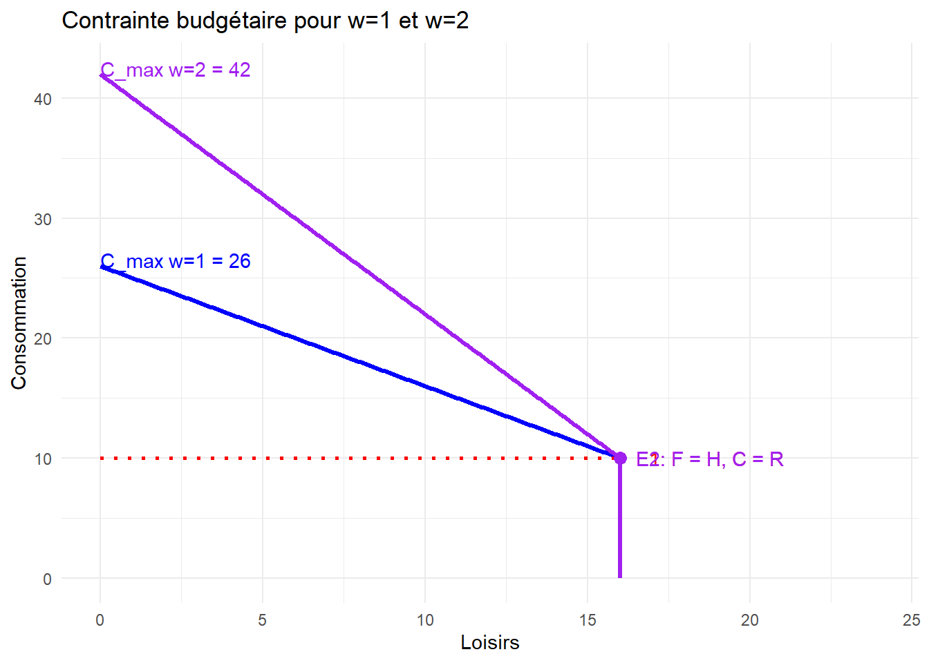
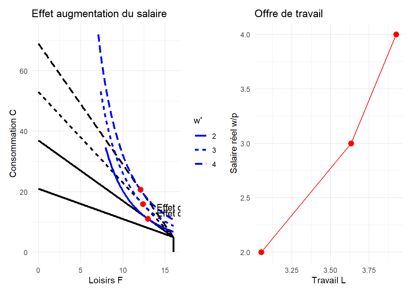
Déplacement de la contraite quand w augmente

Show the code

library(ggplot2)

# Paramètres
H <- 16
R <- 10
F_max <- 24

# Domaine pour la pente
F_vals <- seq(0, H, length.out = 300)

# Contrainte pour w = 1
w1 <- 1
C_vals1 <- w1*H + R - w1*F_vals
df_pente1 <- data.frame(F = F_vals, C = C_vals1)

F_E1 <- H
C_E1 <- R  # = w1*H + R - w1*H
C_max1 <- w1*H + R

# Contrainte pour w = 2
w2 <- 2
C_vals2 <- w2*H + R - w2*F_vals
df_pente2 <- data.frame(F = F_vals, C = C_vals2)

F_E2 <- H
C_E2 <- R  # = w2*H + R - w2*H
C_max2 <- w2*H + R

# Tracé
ggplot() +
  # Droite de la contrainte w=1
  geom_line(data = df_pente1, aes(x = F, y = C), color = "blue", size = 1.2) +
  # Segment vertical bleu w=1
  geom_segment(aes(x = F_E1, xend = F_E1, y = 0, yend = C_E1), color = "blue", size = 1.2) +
  # Segment horizontal pointillé rouge w=1
  geom_segment(aes(x = 0, xend = F_E1, y = C_E1, yend = C_E1), color = "red", linetype = "dotted", size = 1) +
  # Point E1
  geom_point(aes(x = F_E1, y = C_E1), color = "red", size = 3) +
  annotate("text", x = F_E1 + 0.5, y = C_E1, label = paste0("E1: F = H, C = R"), color = "red", hjust = 0) +
  
  # Droite de la contrainte w=2
  geom_line(data = df_pente2, aes(x = F, y = C), color = "purple", size = 1.2) +
  # Segment vertical violet w=2
  geom_segment(aes(x = F_E2, xend = F_E2, y = 0, yend = C_E2), color = "purple", size = 1.2) +
  # Segment horizontal pointillé rouge w=2
  geom_segment(aes(x = 0, xend = F_E2, y = C_E2, yend = C_E2), color = "red", linetype = "dotted", size = 1) +
  # Point E2
  geom_point(aes(x = F_E2, y = C_E2), color = "purple", size = 3) +
  annotate("text", x = F_E2 + 0.5, y = C_E2, label = paste0("E2: F = H, C = R"), color = "purple", hjust = 0) +

  # Annotation pour C intercept w=1
  annotate("text", x = 0, y = C_max1 + 0.5, label = paste0("C_max w=1 = ", C_max1), color = "blue", hjust = 0) +
  # Annotation pour C intercept w=2
  annotate("text", x = 0, y = C_max2 + 0.5, label = paste0("C_max w=2 = ", C_max2), color = "purple", hjust = 0) +
  
  labs(
    title = "Contrainte budgétaire pour w=1 et w=2",
    x = "Loisirs",
    y = "Consommation"
  ) +
  scale_x_continuous(limits = c(0, F_max)) +
  theme_minimal()

Show the code

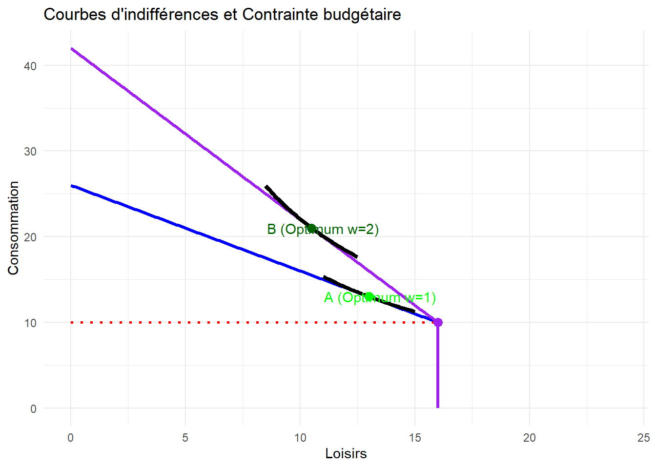
library(ggplot2)

# Paramètres
H <- 16
R <- 10
F_max <- 24
beta <- 0.5

# Contraintes
w1 <- 1
w2 <- 2

# Droites de contrainte
F_vals1 <- seq(0, H, length.out = 300)
C_vals1 <- w1*H + R - w1*F_vals1
df_pente1 <- data.frame(F = F_vals1, C = C_vals1)

F_vals2 <- seq(0, H, length.out = 300)
C_vals2 <- w2*H + R - w2*F_vals2
df_pente2 <- data.frame(F = F_vals2, C = C_vals2)

# Points E
F_E1 <- H; C_E1 <- R
F_E2 <- H; C_E2 <- R

# Optimums Cobb-Douglas
C_max1 <- w1*H + R
C_A <- beta * C_max1
F_A <- (1-beta) * C_max1 / w1
U_A <- C_A^beta * F_A^(1-beta)

C_max2 <- w2*H + R
C_B <- beta * C_max2
F_B <- (1-beta) * C_max2 / w2
U_B <- C_B^beta * F_B^(1-beta)

# Mini segments convexe autour des optimums
delta <- 2  # largeur en Loisirs
F_indiff_A <- seq(F_A - delta, F_A + delta, length.out = 50)
C_indiff_A <- (U_A / F_indiff_A^(1-beta))^(1/beta)
df_indiff_A <- data.frame(F = F_indiff_A, C = C_indiff_A)

F_indiff_B <- seq(F_B - delta, F_B + delta, length.out = 50)
C_indiff_B <- (U_B / F_indiff_B^(1-beta))^(1/beta)
df_indiff_B <- data.frame(F = F_indiff_B, C = C_indiff_B)

# Tracé
ggplot() +
  # Contraintes
  geom_line(data = df_pente1, aes(x = F, y = C), color = "blue", size = 1.2) +
  geom_segment(aes(x = F_E1, xend = F_E1, y = 0, yend = C_E1), color = "blue", size = 1.2) +
  geom_segment(aes(x = 0, xend = F_E1, y = C_E1, yend = C_E1), color = "red", linetype = "dotted", size = 1) +

  geom_line(data = df_pente2, aes(x = F, y = C), color = "purple", size = 1.2) +
  geom_segment(aes(x = F_E2, xend = F_E2, y = 0, yend = C_E2), color = "purple", size = 1.2) +
  geom_segment(aes(x = 0, xend = F_E2, y = C_E2, yend = C_E2), color = "red", linetype = "dotted", size = 1) +

  # Points E
  geom_point(aes(x = F_E1, y = C_E1), color = "red", size = 3) +
  geom_point(aes(x = F_E2, y = C_E2), color = "purple", size = 3) +

  # Courbes d'indifférence convexes (mini segments)
  geom_line(data = df_indiff_A, aes(x = F, y = C), color = "black",  size = 1.5) +
  geom_line(data = df_indiff_B, aes(x = F, y = C), color = "black" , size = 1.5) +

  # Points optimum
  geom_point(aes(x = F_A, y = C_A), color = "green", size = 3) +
  geom_point(aes(x = F_B, y = C_B), color = "darkgreen", size = 3) +

  # Annotations
  annotate("text", x = F_A + 0.5, y = C_A, label = "A (Optimum w=1)", color = "green") +
  annotate("text", x = F_B + 0.5, y = C_B, label = "B (Optimum w=2)", color = "darkgreen") +

  labs(title = "Courbes d'indifférences et Contrainte budgétaire",
       x = "Loisirs", y = "Consommation") +
  scale_x_continuous(limits = c(0, F_max)) +
  theme_minimal()

Show the code

library(ggplot2)

# Paramètres
H <- 16
R <- 10
w <- 1
w_prime <- 2  # nouveau salaire
p <- 1

# Contrainte initiale
F_vals <- seq(0,H,length.out=200)
C_vals <- (w*H + R - w*F_vals)/p
df_constr <- data.frame(F=F_vals, C=C_vals)
df_vert <- data.frame(F=H, C=seq(0,R,length.out=50))

# Contrainte après augmentation w -> w'
C_vals_prime <- (w_prime*H + R - w_prime*F_vals)/p
df_constr_prime <- data.frame(F=F_vals, C=C_vals_prime)

# Optimum initial
F_star <- (w*H + R)/(2*w)
C_star <- (w*H + R)/(2*p)
U_star <- F_star * C_star

# Optimum après w'
F_star_prime <- (w_prime*H + R)/(2*w_prime)
C_star_prime <- (w_prime*H + R)/(2*p)
U_star_prime <- F_star_prime * C_star_prime

# Courbes d'indifférence
delta <- 5
F_CI <- seq(max(0,F_star-delta), min(H,F_star+delta), length.out=100)
C_CI <- U_star / F_CI
df_CI <- data.frame(F=F_CI, C=C_CI)

F_CI_prime <- seq(max(0,F_star_prime-delta), min(H,F_star_prime+delta), length.out=100)
C_CI_prime <- U_star_prime / F_CI_prime
df_CI_prime <- data.frame(F=F_CI_prime, C=C_CI_prime)

# Tracé
ggplot() +
  geom_line(data=df_constr, aes(F,C), color="black", size=1.2) +
  geom_line(data=df_constr_prime, aes(F,C), color="black", linetype="dashed", size=1.2) +
  geom_line(data=df_vert, aes(F,C), color="black", size=1.2) +
  geom_line(data=df_CI, aes(F,C), color="blue", size=1.5) +
  geom_line(data=df_CI_prime, aes(F,C), color="blue", size=1.5, linetype="dashed") +
  geom_point(aes(F_star, C_star), color="red", size=3) +
  geom_point(aes(F_star_prime, C_star_prime), color="red", size=3, shape=17) +
  annotate("text", x=F_star+0.5, y=C_star, label="A", color="red") +
  annotate("text", x=F_star_prime+0.5, y=C_star_prime, label="A'", color="red") +
  labs(title="Effet augmentation du salaire : w → w'", x="Loisirs F", y="Consommation C") +
  theme_minimal()

Construction de la courbe d’offre de travail

Show the code

library(ggplot2)
library(patchwork)

# Paramètres
H <- 16
w <- 1
R <- 5
p <- 1

# Différents nouveaux salaires
w_primes <- c(2, 3, 4) # plusieurs scénarios

# Contrainte initiale
F_vals <- seq(0, H, length.out = 200)
C_vals <- (w*H + R - w*F_vals)/p
df_constr <- data.frame(F = F_vals, C = C_vals)

# Segment vertical pour dotation
df_vert <- data.frame(F = H, C = seq(0, R, length.out = 50))

# Fonction pour calculer optimum et courbe d'indifférence
calc_opt_CI <- function(w_new){
  F_star <- min(0.7*(w_new*H + R)/w_new, H)
  C_star <- 0.3*(w_new*H + R)/p
  U_star <- C_star^0.3 * F_star^0.7
  
  delta <- 5
  F_CI <- seq(max(0,F_star-delta), min(H,F_star+delta), length.out=100)
  C_CI <- (U_star / F_CI^0.7)^(1/0.3)
  df_CI <- data.frame(F=F_CI, C=C_CI, w_new=w_new, F_star=F_star, C_star=C_star)
  
  # Contrainte
  C_vals_new <- (w_new*H + R - w_new*F_vals)/p
  df_constr_new <- data.frame(F=F_vals, C=C_vals_new, w_new=w_new)
  
  return(list(df_CI=df_CI, df_constr=df_constr_new))
}

# Boucle sur les nouveaux salaires
list_CI <- list()
list_constr <- list()
df_opt <- data.frame() # pour les points optimums
for(wp in w_primes){
  res <- calc_opt_CI(wp)
  list_CI[[as.character(wp)]] <- res$df_CI
  list_constr[[as.character(wp)]] <- res$df_constr
  
  df_opt <- rbind(df_opt, data.frame(F_star=res$df_CI$F_star[1], 
                                     C_star=res$df_CI$C_star[1], w_new=wp))
}

df_CI_all <- do.call(rbind, list_CI)
df_constr_all <- do.call(rbind, list_constr)

# Graphe principal : F vs C
g1 <- ggplot() +
  geom_line(data=df_constr, aes(F,C), color="black", size=1.2) +
  geom_line(data=df_vert, aes(F,C), color="black", size=1.2) +
  geom_line(data=df_constr_all, aes(F,C, linetype=factor(w_new)), color="black", size=1.2) +
  geom_line(data=df_CI_all, aes(F,C, linetype=factor(w_new)), color="blue", size=1.2) +
  geom_point(data=df_opt, aes(F_star,C_star), color="red", size=3) +
  annotate("text", x=14, y=15, label="Effet de revenu > effet de substitution", hjust=0, size=4) +
  annotate("text", x=14, y=13, label="Effet de substitution > effet de revenu", hjust=0, size=4) +
  labs(title="Effet augmentation du salaire", x="Loisirs F", y="Consommation C", linetype="w'") +
  theme_minimal()

# Graphe secondaire : Offre de travail (L horizontal, w/p vertical)
df_opt$L <- H - df_opt$F_star
g2 <- ggplot(df_opt, aes(x=L, y=w_new/p)) +
  geom_point(size=3, color="red") +
  geom_line(group=1, color="red") +
  labs(title="Offre de travail", x="Travail L", y="Salaire réel w/p") +
  theme_minimal()

# Combiner les deux graphes
g1 + g2 + plot_layout(ncol=2)