La base de données utilisée porte sur les pratiques culturelles des français, 2018, (Enquête sur les pratiques culturelles des Français, 2018) elle comprend un total de 1572 variables, réparties en plusieurs modules thématiques .
La structure thématique des variables se présente comme suit :
Domaine
Nombre de variables
Variables socio-démographiques
190
Loisirs et vacances
41
Pratiques en amateur
201
Jeux vidéo
29
Films, séries, émissions
287
Information
41
Écoute de musique et d’émissions
109
Bibliothèque et livres
121
Concerts, cinéma, théâtre, danse et festivals
233
Musées, expositions et patrimoine
94
Équipements et internet
29
Situation principale vis-à-vis du travail et activité professionnelle
48
Ressources culturelles
40
Situation dans l’enfance
103
Logement
6
Cette répartition met en évidence la quantité considérable de données relatives aux pratiques culturelles et de loisirs (plus de 1000 variables au total dans ces modules) , qui constitue la base de l’analyse pour la construction des indices de genre continus.
Le nombre total d’individus dans l’échantillon est de 9 234 .
L’échantillon est composé de 4 162 hommes et 5 072 femmes .
On présente une répartition par âge, revenu, satisfaction, niveau de diplôme, situation d’emploi, état de santé et situation de couple. Pour la majorité de ces caractéristiques (âge, revenu, satisfaction, diplôme, situation emploi, santé, couple), des différences statistiquement signifficatives entre hommes et femmes sont notées (p < 0.001 dans la plupart des cas) .
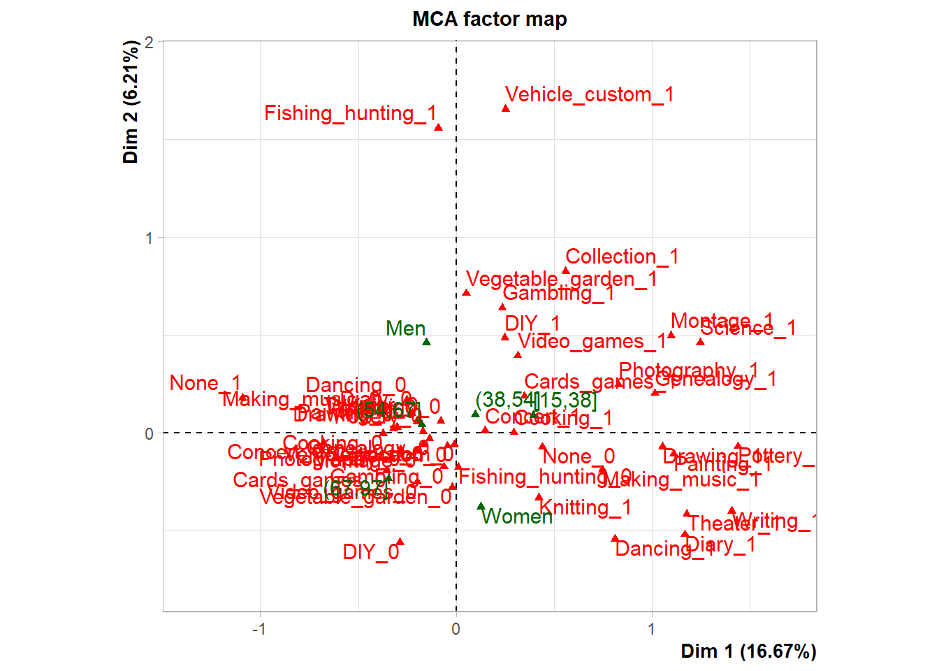
On détaille ensuite la fréquence de participation à diverses pratiques culturelles et en amateur, ventilée par sexe. Ce tableau illustre la différenciation marquée des pratiques selon le genre.
Par exemple : Le tricot (“Knitting”) est pratiqué par 27% des femmes contre seulement 1.8% des hommes (p < 0.001) . Le bricolage (“DIY”) est l’activité de 64% des hommes contre 45% des femmes (p < 0.001) . La pêche/chasse (“Fishing hunting”) est pratiquée par 17% des hommes et 4.2% des femmes (p < 0.001) . Tenir un journal intime (“Diary”) est l’habitude de 24% des femmes contre 6.8% des hommes (p < 0.001) . La danse (“Dancing”) concerne 35% des femmes et 9.9% des hommes (p < 0.001) . Les jeux vidéo (“Video games”) sont pratiqués par 42% des hommes et 36% des femmes (p < 0.001) .
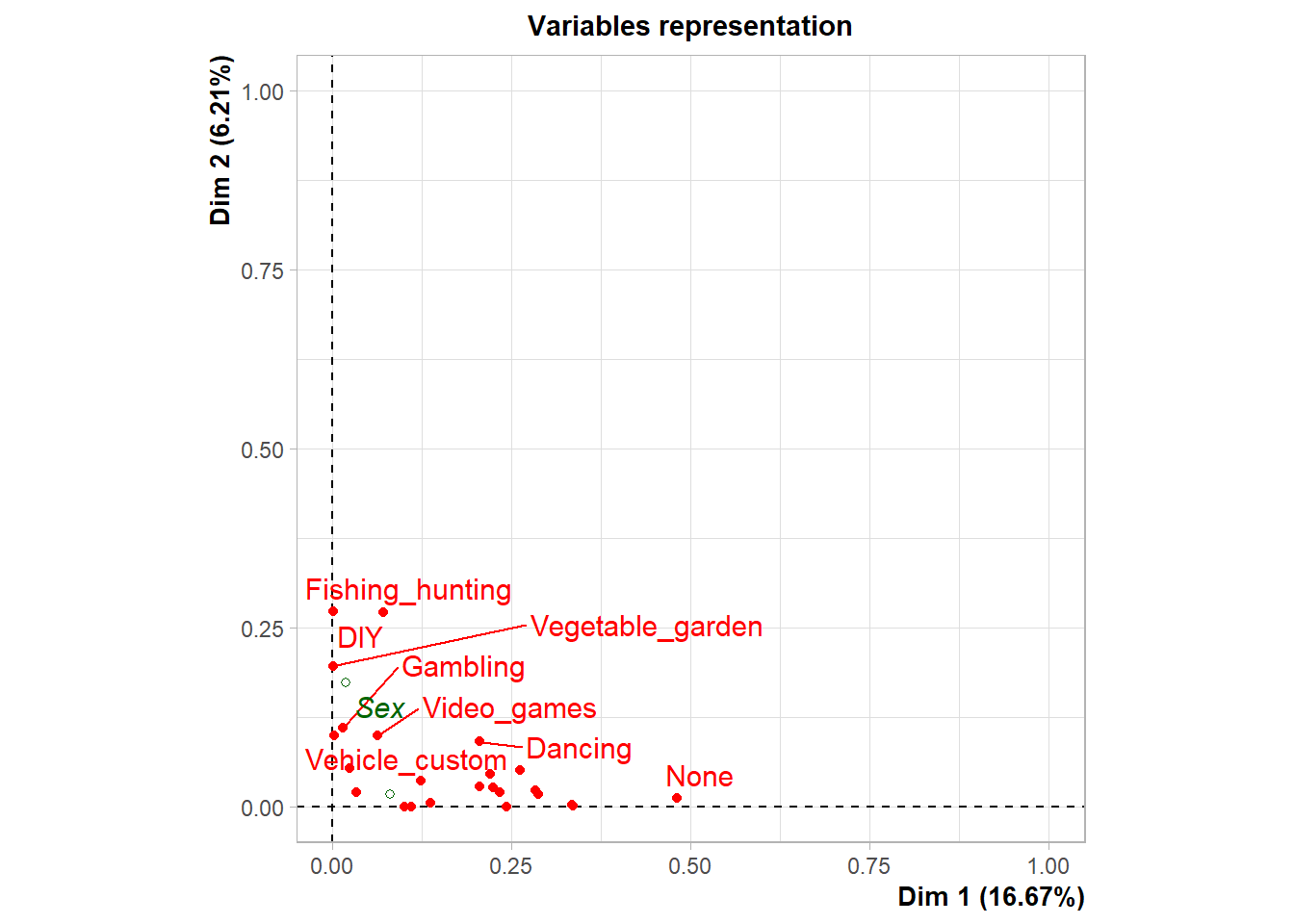
Ces données sur les pratiques culturelles différenciées sont ensuite utilisées pour construire les indices continus de genre, via l’Analyse des Correspondances Multiples (ACM) et la régression LASSO . Les coordonnées obtenues par l’ACM et les coeffcients de la régression LASSO pour différentes variables culturelles sont les poids utilisés pour calculer ces indices.
Lecture: Parmi l’ensemble des individus interrogés, 16% pratiquent le tricot (Knitting); 27% des femmes le pratiquent contre 1,8% des hommes
Encadré Technique 1: Détails de la méthode ACM
L’ACM permet d’explorer les relations entre plusieurs variables qualitatives en projetant les individus et les modalités dans un espace de faible dimension. Elle est souvent utilisée pour analyser des questionnaires et des tableaux de contingence complexes.
Principaux résultats d’une ACM
Inertie totale
Mesure la dispersion des données et est donnée par :
où \(\lambda_k\) sont les valeurs propres et \(q\) est le nombre total de modalités.
Valeurs propres \(\lambda_k\)
Elles indiquent la variance expliquée par chaque axe factoriel. Plus une valeur propre est élevée, plus l’axe correspondant est important dans l’analyse.
Rapports de corrélation \(\eta^2\)
Le rapport de corrélation \(\eta^2\) mesure la liaison entre une variable et un axe factoriel :
où $f_i $ est la fréquence de l’individu/modalité $i $, et \(d_{i,k}\)est sa distance à l’axe \(k\) .
Coordonnées des individus et modalités
Elles sont obtenues à partir des vecteurs propres et permettent la représentation graphique des données :
\(C_{i,k} = \frac{v_{i,k}}{\sqrt{\lambda_k}}\)
où \(v_{i,k}\) est le vecteur propre associé à l’axe \(k\).
Cos² (Qualité de représentation)
Indique dans quelle mesure un point est bien représenté sur un axe donné. Une valeur proche de **1** signifie que la projection sur cet axe est pertinente.
Contributions
Elles mesurent l’importance d’une modalité ou d’un individu dans la construction d’un axe. Plus une contribution est élevée, plus l’élément joue un rôle important dans l’interprétation de l’axe.
# Extract coordinates for dimension 2coord_dim2_modalites <- acm2_fm$var$coord[, 2]# Create a table associating the modalities and their coordinates in dimension 2modalites_coord <-data.frame(Modalite = modalites_names, Coord_Dim2 = coord_dim2_modalites)# Keep only the two necessary columnsmodalites_coord_selected <- modalites_coord[, c("Modalite", "Coord_Dim2")]print(modalites_coord_selected)
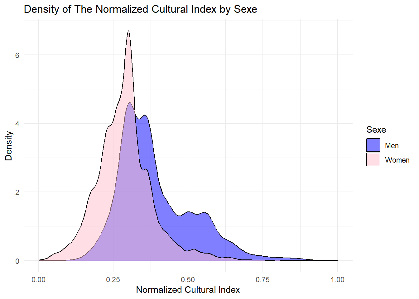
# Initialize a vector to store the index of each individualdata_pratiques$indice_culturel <-0# Browse each individualfor (i in1:nrow(data_pratiques)) {# Initialize individual's index to 0 indice_individu <-0# Browse each practice column (columns 3 to 27)for (pratique in3:27) {# Retrieve the individual's response for this practice (0 or 1) reponse <- data_pratiques[i, pratique]# If the answer is 1, add the coordinate of the corresponding modality to the index.if (reponse ==1) {# Create the modality name (e.g. “knitting_1” or “knitting_0”) nom_modalite_1 <-paste0(names(data_pratiques)[pratique], "_1") nom_modalite_0 <-paste0(names(data_pratiques)[pratique], "_0")# Find the coordinate associated with the corresponding modalityif (nom_modalite_1 %in% modalites_coord$Modalite) { indice_individu <- indice_individu + modalites_coord$Coord_Dim2[modalites_coord$Modalite == nom_modalite_1] }if (nom_modalite_0 %in% modalites_coord$Modalite) { indice_individu <- indice_individu + modalites_coord$Coord_Dim2[modalites_coord$Modalite == nom_modalite_0] } } }# Assign the calculated index to the individual data_pratiques$indice_culturel[i] <- indice_individu}####Normalisation# Calculate minimum and maximum index valuesmin_indice <-min(data_pratiques$indice_culturel, na.rm =TRUE)max_indice <-max(data_pratiques$indice_culturel, na.rm =TRUE)# Normalize indexdata_pratiques$indice_culturel_normalise <- (data_pratiques$indice_culturel - min_indice) / (max_indice - min_indice)# Check resultshead(data_pratiques[, c("indice_culturel", "indice_culturel_normalise")])
Notre indice est donc construit de la façon suivante:
\[I_{1j} = \sum_{k=1}^{Z} w_{1k} \cdot X_{k j}\]
Dans cette expression, \(I_{1j}\) désigne l’indice de l’individu \(j\), tandis que \(w_{1k}\) représente le poids associé à chaque variable culturelle \(X_{kj}\). La somme englobe toutes les variables culturelles \(Z\), ce qui nous permet de saisir l’engagement culturel global de l’individu.
code R
my_data_frame$identity<-data_pratiques$indice_culturel_normalisemy_data_frame$indice<-ra_data$indice_culturelggplot(my_data_frame, aes(x = identity, fill = Sex)) +geom_density(alpha =0.5) +scale_fill_manual(values =c("blue", "pink")) +labs(title ="Density of The Normalized Cultural Index by Sexe",x ="Normalized Cultural Index",y ="Density",fill ="Sexe") +theme_minimal()
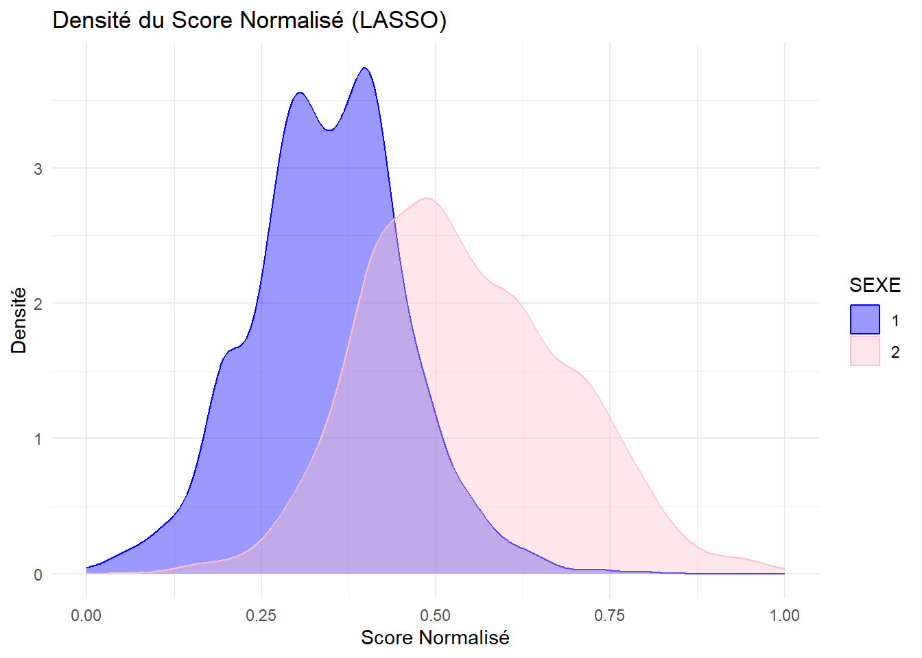
La régression LASSO (Least Absolute Shrinkage and Selection Operator) est une méthode de régression pénalisée qui sélectionne automatiquement les variables les plus pertinentes en contraignant la somme des valeurs absolues des coefficients. Dans notre analyse, nous avons utilisé la régression LASSO avec validation croisée sur un ensemble d’activités culturelles pour prédire le sexe des individus (homme ou femme).
Les variables ayant des coeffcients non nuls après régularisation ont été retenues. Un score linéaire a ensuite été calculé pour chaque individu sous la forme : \[
\text{IndiceLASSO} = \sum_{j \in S} \beta_j \, x_j
\] où S est l’ensemble des variables sélectionnées, βj leur coefficient estimé, et xj la valeur observée de la variable pour un individu donné. Cet indice est ensuite normalisé entre 0 et 1 pour faciliter l’interprétation. Il reflète le positionnement d’un individu sur une dimension latente déterminée automatiquement par les pratiques différenciatrices selon le sexe.
code R
### 1️⃣ Préparation des données ----library(glmnet)library(ggplot2)# Liste des variablesvars <-c("SEXE", "Knitting", "Cards_games", "Gambling", "Cooking", "DIY","Vegetable_garden", "Ornamental_garden", "Fishing_hunting", "Collection","Vehicle_custom", "Making_music", "Diary", "Writing", "Painting", "Montage","Circus", "Pottery", "Theater", "Drawing", "Dancing", "Photography","Genealogy", "Science", "None", "No_Amateur", "Video_games", "TV","Radio", "Library", "Museums", "Internet", "Concert")# Sous-ensemble des variablesdf_subset <- my_data_frame[, vars]# Remplacer NA par 0 dans les variables explicativesdf_subset[,-1] <-lapply(df_subset[,-1], function(x) { x[is.na(x)] <-0; x })# Convertir SEXE en facteur binairedf_subset$SEXE <-as.factor(df_subset$SEXE)# Split train / testset.seed(123)n <-nrow(df_subset)train_index <-sample(seq_len(n), size =floor(2*n/3))train_data <- df_subset[train_index, ]test_data <- df_subset[-train_index, ]### 2️⃣ Matrices X et y ----x_train <-model.matrix(SEXE ~ ., data = train_data)[, -1]y_train <- train_data$SEXEx_test <-model.matrix(SEXE ~ ., data = test_data)[, -1]y_test <- test_data$SEXE### 3️⃣ LASSO avec CV ----cv_lasso <-cv.glmnet(x_train, y_train, alpha =1, family ="binomial")best_lambda <- cv_lasso$lambda.mincat("Meilleur lambda :", best_lambda, "\n")
Meilleur lambda : 0.0007031016
code R
# Coefficients non nulscoef_lasso <-coef(cv_lasso, s ="lambda.min")coeffs_df <-data.frame(Variable =rownames(as.matrix(coef_lasso)),Coefficient =as.numeric(coef_lasso))coeffs_nz <-subset(coeffs_df, Coefficient !=0& Variable !="(Intercept)")print(coeffs_nz)
# ✅ 1. On garde uniquement les variables présentes à la fois dans les coeffs et dans my_data_framevars_kept <-intersect(coeffs_nz$Variable, colnames(my_data_frame))# ✅ 2. Sous‐ensemble de la matrice de donnéesx_full_reduced <- my_data_frame[, vars_kept, drop =FALSE]# ✅ 3. Vecteur des coefficients dans le même ordre que les variables conservéescoef_vector <- coeffs_nz$Coefficient[match(vars_kept, coeffs_nz$Variable)]# ✅ 4. Calcul du score brut LASSOmy_data_frame$score_LASSO <-as.numeric(as.matrix(x_full_reduced) %*% coef_vector)# ✅ 5. Normalisation du scoremin_s <-min(my_data_frame$score_LASSO, na.rm =TRUE)max_s <-max(my_data_frame$score_LASSO, na.rm =TRUE)my_data_frame$score_normalise_LASSO <-if (max_s > min_s) { (my_data_frame$score_LASSO - min_s) / (max_s - min_s)} else {0}
code R
predictor_var <- my_data_frame$score_LASSO# List of cultural activitiescultural_activities <-c("Knitting" , "Cards_games", "Gambling" , "Cooking" , "DIY" ,"Vegetable_garden" , "Fishing_hunting" , "Collection" ,"Vehicle_custom","Making_music" ,"Diary" ,"Writing" , "Painting", "Montage" , "Pottery" , "Theater" , "Drawing" , "Dancing", "Photography" ,"Genealogy" , "Science" ,"None" ,"Video_games" ,"Library" ,"Concert")# Initialiser un tableau vide pour les résultatsresult_table <-data.frame(Activity =character(), Accuracy =numeric(), stringsAsFactors =FALSE)# Boucle sur chaque activité culturellefor (activity in cultural_activities) {# Créer la formule du modèle model_formula <-as.formula(paste(activity, "~ score_LASSO"))# Estimer le modèle Probit model <-glm(model_formula, data = my_data_frame, family =binomial(link ="probit"))# Prédictions predicted <-ifelse(predict(model, type ="response") >=0.5, 1, 0)# Calcul de l'exactitude correct_predictions <-sum(predicted == my_data_frame[[activity]], na.rm =TRUE) total_predictions <-nrow(my_data_frame) accuracy <- (correct_predictions / total_predictions) *100# Ajouter la ligne au tableau de résultats result_table[nrow(result_table) +1, ] <-list(Activity = activity, Accuracy = accuracy)}# Afficher le tableau finalprint(result_table)
# Proportions de 'score_scale' par genretable_score_gender <-table(my_data_frame$score_scale, my_data_frame$Sex)table_score_gender_percent <-prop.table(table_score_gender, 2) *100# Calcul par genretable_score_gender_percent
                         Men       Women
  Very Masculine  2.66240682  0.06116208
  1              19.80830671  1.16207951
  2              46.96485623 13.63914373
  3              26.73056443 36.33027523
  4               3.40788072 31.43730887
  5               0.31948882 13.70030581
  Very Feminine   0.10649627  3.66972477
code R
# Proportions de 'satisfaction' par genretable_satisfaction_gender <-table(my_data_frame$satisfaction, my_data_frame$Sex)table_satisfaction_gender_percent <-prop.table(table_satisfaction_gender, 2) *100# Calcul par genretable_satisfaction_gender_percent
              Men    Women
  High   35.15399 32.66917
  Low    35.80366 39.75143
  Medium 29.04235 27.57940
code R
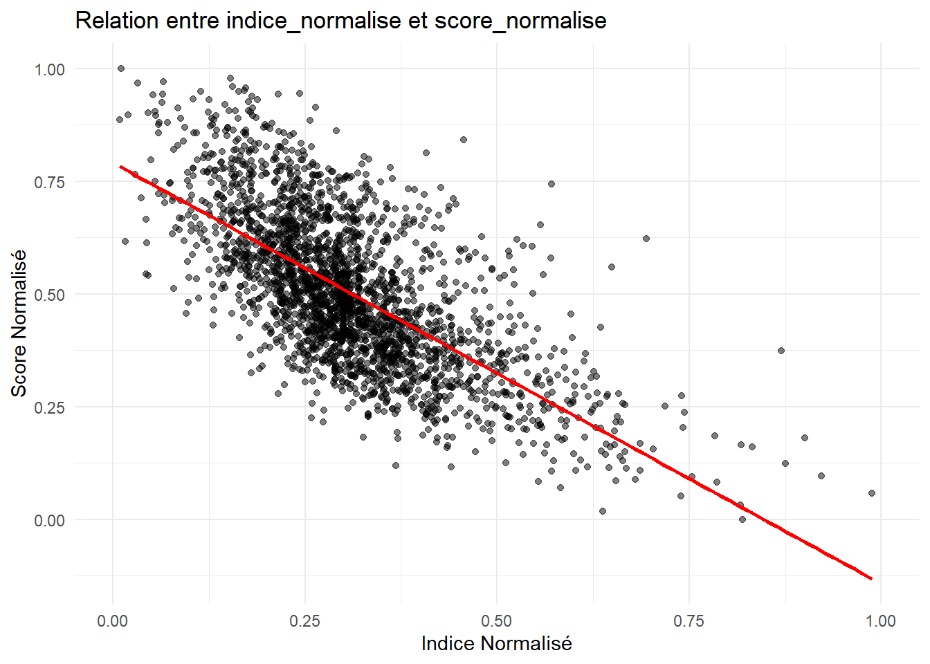
# Visualiser la relation entre indice_normalise et score_normaliselibrary(ggplot2)ggplot(my_data_frame, aes(x = identity, y = score_normalise_LASSO)) +geom_point(alpha =0.5) +labs(title ="Relation entre indice_normalise et score_normalise", x ="Indice Normalisé", y ="Score Normalisé") +theme_minimal() +geom_smooth(method ="lm", col ="red", se =FALSE) # Ajouter une droite de régression linéaire
code R
# Convertir les variables en facteurs si nécessairemy_data_frame$DIPLOM <-as.factor(my_data_frame$DIPLOM)my_data_frame$SEXE <-as.factor(my_data_frame$SEXE)my_data_frame$CLASSIF <-as.factor(my_data_frame$CLASSIF)my_data_frame$Income <-as.factor(my_data_frame$Income)my_data_frame$Health <-as.factor(my_data_frame$Health)my_data_frame$satisfaction <-as.factor(my_data_frame$satisfaction)my_data_frame$SITUA <-as.factor(my_data_frame$SITUA)my_data_frame$CS2D <-as.factor(my_data_frame$CS2D)# Créer une fonction pour comparer les modèles avec 'score' et 'Sex' comme prédicteurscompare_models <-function(variable) {# Affichage de la variable actuellement traitéecat("Traitement de la variable :", variable, "\n")# Modèle avec score comme prédicteur model_score <-polr(as.formula(paste(variable, "~ score_normalise_LASSO")), data = my_data_frame, method ="logistic")# Modèle avec sexe comme prédicteur model_sex <-polr(as.formula(paste(variable, "~ SEXE")), data = my_data_frame, method ="logistic")# Comparer l'AIC des deux modèles aic_score <-AIC(model_score) aic_sex <-AIC(model_sex)# Comparer et retourner le meilleur modèleif (aic_score < aic_sex) {return(data.frame(variable = variable, best_predictor ="Score", AIC_score = aic_score, AIC_sex = aic_sex)) } else {return(data.frame(variable = variable, best_predictor ="Sex", AIC_score = aic_score, AIC_sex = aic_sex)) }}# Liste des variables d'intérêt à analyservariables <-c("DIPLOM", "CLASSIF", "SITUA", "satisfaction", "Health", "Income", "CS2D")# Appliquer la fonction pour chaque variable d'intérêt et combiner les résultatsresults <-do.call(rbind, lapply(variables, compare_models))
Traitement de la variable : DIPLOM
Traitement de la variable : CLASSIF
Traitement de la variable : SITUA
Traitement de la variable : satisfaction
Traitement de la variable : Health
Traitement de la variable : Income
Traitement de la variable : CS2D
code R
# Afficher les résultats sous forme de tableauprint(results)
# Convertir les variables en facteurs si nécessairemy_data_frame$DIPLOM <-as.factor(my_data_frame$DIPLOM)my_data_frame$SEXE <-as.factor(my_data_frame$SEXE)my_data_frame$CLASSIF <-as.factor(my_data_frame$CLASSIF)my_data_frame$Income <-as.factor(my_data_frame$Income)my_data_frame$Health <-as.factor(my_data_frame$Health)my_data_frame$satisfaction <-as.factor(my_data_frame$satisfaction)my_data_frame$SITUA <-as.factor(my_data_frame$SITUA)my_data_frame$CS2D <-as.factor(my_data_frame$CS2D)# Créer une fonction pour comparer les modèles avec 'score' et 'Sex' comme prédicteurscompare_models <-function(variable) {# Affichage de la variable actuellement traitéecat("Traitement de la variable :", variable, "\n")# Modèle avec score comme prédicteur model_score <-polr(as.formula(paste(variable, "~ score_normalise_LASSO")), data = my_data_frame, method ="logistic")# Modèle avec sexe comme prédicteur model_id <-polr(as.formula(paste(variable, "~ identity")), data = my_data_frame, method ="logistic")# Comparer l'AIC des deux modèles aic_score <-AIC(model_score) aic_id <-AIC(model_id)# Comparer et retourner le meilleur modèleif (aic_score < aic_id) {return(data.frame(variable = variable, best_predictor ="Score", AIC_score = aic_score, AIC_id = aic_id)) } else {return(data.frame(variable = variable, best_predictor ="id", AIC_score = aic_score, AIC_id = aic_id)) }}# Liste des variables d'intérêt à analyservariables <-c("satisfaction", "Health", "Income")# Appliquer la fonction pour chaque variable d'intérêt et combiner les résultatsresults <-do.call(rbind, lapply(variables, compare_models))
Traitement de la variable : satisfaction
Traitement de la variable : Health
Traitement de la variable : Income
code R
# Afficher les résultats sous forme de tableauprint(results)
      variable best_predictor AIC_score   AIC_id
1 satisfaction          Score  5550.873 20142.02
2       Health          Score  3288.556 14580.80
3       Income          Score  4835.411 17466.37
4.5 Variables socio-économiques et score de genre
4.5.1 Femmes:
code R
df_femmes <- my_data_frame %>%filter(Sex =="Women")# Choix des variables explicativesgroup_vars <-c("Income", "age_group", "DIPLOMA", "Health")# Créer un tableau avec score_scale en colonnes et les variables explicatives en lignestable_lasso_femmes_inverse <- df_femmes %>%tbl_summary(by = score_scale, # score_scale en colonnesinclude =all_of(group_vars), # variables explicatives en lignesstatistic =all_categorical() ~"{p}%",missing ="no" )%>%add_p()table_lasso_femmes_inverse
Characteristic
Very Masculine N = 11
1 N = 191
2 N = 2231
3 N = 5941
4 N = 5141
5 N = 2241
Very Feminine N = 601
p-value
Income
High
0%
33%
39%
40%
42%
41%
38%
Low
0%
28%
28%
23%
24%
26%
30%
Medium
100%
39%
34%
37%
34%
34%
32%
age_group
[15-38[
0%
37%
30%
30%
29%
33%
28%
[38-54[
0%
32%
34%
36%
35%
26%
30%
[54-67[
100%
26%
28%
28%
29%
35%
33%
[67-97[
0%
5.3%
7.6%
6.6%
7.0%
6.3%
8.3%
DIPLOMA
Bac général / technologique
0%
11%
16%
18%
17%
16%
22%
Bac professionnel / équivalent
0%
16%
6.3%
4.2%
4.5%
3.6%
3.3%
Bac+2 à Bac+5 (hors doctorat)
100%
21%
43%
42%
48%
54%
57%
CAP / BEP
0%
16%
16%
15%
14%
9.4%
6.7%
Capacité / DAEU / ESEU
0%
0%
0.5%
0.3%
0.4%
0.4%
0%
CEP / Brevet / DNB
0%
16%
11%
14%
13%
12%
10%
Doctorat
0%
0%
2.3%
1.0%
1.0%
1.8%
1.7%
Sans diplôme
0%
21%
5.0%
4.7%
2.9%
3.6%
0%
Health
Bad
0%
0%
7.7%
5.2%
4.9%
6.7%
5.0%
Good
100%
84%
77%
79%
77%
75%
70%
Medium
0%
16%
16%
16%
18%
18%
25%
1
4.5.2 Hommes:
code R
df_hommes <- my_data_frame %>%filter(Sex =="Men")# Choix des variables explicativesgroup_vars <-c("Income", "age_group", "DIPLOMA", "Health")# Créer un tableau avec score_scale en colonnes et les variables explicatives en lignestable_lasso_hommes_inverse <- df_hommes %>%tbl_summary(by = score_scale, # score_scale en colonnesinclude =all_of(group_vars), # variables explicatives en lignesstatistic =all_categorical() ~"{p}%",missing ="no" ) %>%add_p()table_lasso_hommes_inverse
Characteristic
Very Masculine N = 251
1 N = 1861
2 N = 4411
3 N = 2511
4 N = 321
5 N = 31
Very Feminine N = 11
p-value
Income
High
55%
47%
49%
42%
63%
100%
100%
Low
18%
15%
17%
21%
10%
0%
0%
Medium
27%
38%
34%
37%
27%
0%
0%
age_group
[15-38[
40%
39%
27%
30%
38%
33%
0%
[38-54[
36%
37%
32%
35%
22%
67%
0%
[54-67[
20%
22%
34%
28%
25%
0%
0%
[67-97[
4.0%
3.2%
7.5%
6.8%
16%
0%
100%
DIPLOMA
Bac général / technologique
8.0%
13%
16%
12%
9.4%
33%
0%
Bac professionnel / équivalent
8.0%
5.9%
7.3%
8.0%
3.1%
0%
0%
Bac+2 à Bac+5 (hors doctorat)
32%
45%
42%
48%
63%
67%
100%
CAP / BEP
24%
16%
20%
15%
6.3%
0%
0%
Capacité / DAEU / ESEU
0%
0.5%
0.2%
0%
0%
0%
0%
CEP / Brevet / DNB
24%
15%
9.3%
10%
3.1%
0%
0%
Doctorat
0%
1.6%
2.7%
3.2%
9.4%
0%
0%
Sans diplôme
4.0%
2.7%
3.2%
4.0%
6.3%
0%
0%
Health
Bad
0%
2.2%
5.3%
6.4%
6.3%
0%
0%
Good
88%
85%
82%
76%
81%
100%
100%
Medium
12%
13%
13%
17%
13%
0%
0%
1
4.6 Distance aux normes
code R
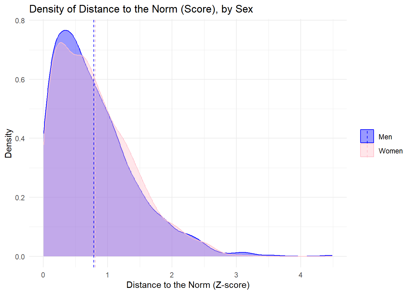
library(dplyr)library(ggplot2)# S'assurer que SEXE est bien un facteur clairmy_data_frame$Sex <-factor(my_data_frame$Sex, levels =c("Men", "Women"))# Calcul direct du z-score par groupe (pas de jointure)my_data_frame <- my_data_frame %>%group_by(Sex) %>%mutate(mean_gender =mean(score_normalise_LASSO, na.rm =TRUE),sd_gender =sd(score_normalise_LASSO, na.rm =TRUE),distance_abs =abs((score_normalise_LASSO - mean_gender) / sd_gender) ) %>%ungroup()# Calcul des moyennes des distances par sexemean_distances <- my_data_frame %>%group_by(Sex) %>%summarise(mean_distance =mean(distance_abs, na.rm =TRUE),.groups ="drop" )# Visualisationggplot(my_data_frame, aes(x = distance_abs, color = Sex, fill = Sex)) +geom_density(alpha =0.4) +labs(title ="Density of Distance to the Norm (Score), by Sex",x ="Distance to the Norm (Z-score)",y ="Density" ) +scale_fill_manual(values =c("blue", "pink")) +scale_color_manual(values =c("blue", "pink")) +theme_minimal() +geom_vline(data = mean_distances,aes(xintercept = mean_distance, color = Sex),linetype ="dashed" ) +theme(legend.title =element_blank())
code R
library(dplyr)library(ggplot2)library(plotly)# Convertir DIPLOM et Sex en facteursmy_data_frame$DIPLOM <-as.factor(my_data_frame$DIPLOM)my_data_frame$Sex <-as.factor(my_data_frame$Sex)# Création des quartiles de distance_absmy_data_frame <- my_data_frame %>%mutate(quartile_distance =cut(distance_abs, breaks =quantile(distance_abs, probs =c(0, 0.25, 0.5, 0.75, 1), na.rm =TRUE), include.lowest =TRUE, labels =c("Q1", "Q2", "Q3", "Q4"))) # Étiquettes des quartiles# Créer un tableau de proportionsdf_proportions <- my_data_frame %>%group_by(Sex, DIPLOM, quartile_distance) %>%summarise(count =n(), .groups ="drop") %>%group_by(Sex, DIPLOM) %>%mutate(proportion = count /sum(count)) # Calcul de la proportion# Ajouter une colonne avec les descriptions des diplômesdiplome_labels <-c("Vous n'avez jamais été à l'école ou vous l'avez quittée avant la fin du primaire","Aucun diplôme et scolarité interrompue à la fin du primaire ou avant la fin du collège","Aucun diplôme et scolarité jusqu'à la fin du collège et au-delà","CEP","BEPC, brevet élémentaire, brevet des collèges, DNB","CAP, BEP ou diplôme équivalent","Baccalauréat général ou technologique, brevet supérieur","Capacité en droit, DAEU, ESEU","Baccalauréat professionnel, brevet professionnel, de technicien ou d'enseignement, diplôme équivalent","BTS, DUT, DEUST, diplôme de la santé ou social de niveau Bac+2 ou diplôme équivalent","Licence, licence pro, maîtrise ou autre diplôme de niveau Bac+3 ou 4 ou diplôme équivalent","Master, DEA, DESS, diplôme grande école de niveau Bac+5, doctorat de santé","Doctorat de recherche (hors santé)","NSP","REF")# Ajouter les libellés des diplômes à df_proportionsdf_proportions <- df_proportions %>%mutate(DIPLOM_label = diplome_labels[as.numeric(DIPLOM)])# Séparer les données en deux sous-ensembles (Hommes et Femmes)df_men <- df_proportions %>%filter(Sex =="Men")df_women <- df_proportions %>%filter(Sex =="Women")# Graphique pour les hommesfig_men <-plot_ly(df_men, x =~DIPLOM, y =~proportion, color =~quartile_distance, type ="bar",text =~paste(DIPLOM_label, "<br>", round(proportion*100, 1), "%"), # Affichage du libellé et proportiontextposition ="inside") %>%layout(title ="Proportion de score_scale par niveau de diplôme (Hommes)",xaxis =list(title ="Niveau de diplôme"),yaxis =list(title ="Proportion", tickformat ="%"),barmode ="stack", # Empilement des barreshovermode ="closest") # Afficher les informations les plus proches du survol# Graphique pour les femmesfig_women <-plot_ly(df_women, x =~DIPLOM, y =~proportion, color =~quartile_distance, type ="bar",text =~paste(DIPLOM_label, "<br>", round(proportion*100, 1), "%"), # Affichage du libellé et proportiontextposition ="inside") %>%layout(title ="Proportion de score_scale par niveau de diplôme (Femmes)",xaxis =list(title ="Niveau de diplôme"),yaxis =list(title ="Proportion", tickformat ="%"),barmode ="stack", # Empilement des barreshovermode ="closest") # Afficher les informations les plus proches du survol# Afficher les deux graphiques séparésfig_men
code R
fig_women
4.7 Variables Socio-éco et influence sur le score de Genre
              Df Sum Sq Mean Sq F value   Pr(>F)
DIPLOMA        7   0.69 0.09917   3.628 0.000677 ***
SITUA_lab      7   0.82 0.11754   4.300 9.78e-05 ***
Income         2   0.52 0.25892   9.471 8.02e-05 ***
age_group      3   0.09 0.03036   1.110 0.343547
Residuals   2247  61.43 0.02734
---
Signif. codes:  0 '***' 0.001 '**' 0.01 '*' 0.05 '.' 0.1 ' ' 1
6967 observations effacées parce que manquantes
code R
# Installer les packages si nécessaire# install.packages("plotly")# install.packages("dplyr")library(plotly)library(dplyr)# -----------------------------# 1️⃣ ANOVA multi-facteurs# -----------------------------anova_model <-aov(score_normalise_LASSO ~ DIPLOMA + SITUA_lab + Income + age_group, data = my_data_frame)summary(anova_model)
              Df Sum Sq Mean Sq F value   Pr(>F)
DIPLOMA        7   0.69 0.09917   3.628 0.000677 ***
SITUA_lab      7   0.82 0.11754   4.300 9.78e-05 ***
Income         2   0.52 0.25892   9.471 8.02e-05 ***
age_group      3   0.09 0.03036   1.110 0.343547
Residuals   2247  61.43 0.02734
---
Signif. codes:  0 '***' 0.001 '**' 0.01 '*' 0.05 '.' 0.1 ' ' 1
6967 observations effacées parce que manquantes
code R
# -----------------------------# 2️⃣ Moyennes par catégorie# -----------------------------categorical_vars <-c("DIPLOMA", "SITUA_lab", "Income", "age_group")mean_tables <-list()for (var in categorical_vars) { mean_tables[[var]] <- my_data_frame %>%group_by(.data[[var]]) %>%summarise(mean_score =mean(score_normalise_LASSO, na.rm =TRUE)) %>%arrange(desc(mean_score))cat("\nMoyennes pour", var, ":\n")print(mean_tables[[var]])}
Moyennes pour DIPLOMA :
# A tibble: 9 × 2
  DIPLOMA                        mean_score
  <chr>                               <dbl>
1 Capacité / DAEU / ESEU              0.526
2 Bac+2 à Bac+5 (hors doctorat)       0.516
3 Bac général / technologique         0.511
4 CEP / Brevet / DNB                  0.500
5 Doctorat                            0.484
6 Sans diplôme                        0.479
7 CAP / BEP                           0.472
8 Bac professionnel / équivalent      0.465
9 <NA>                                0.447

Moyennes pour SITUA_lab :
# A tibble: 10 × 2
   SITUA_lab                                               mean_score
   <chr>                                                        <dbl>
 1 Femme ou homme au foyer                                      0.550
 2 Autre situation d'inactivité                                 0.531
 3 Chômeur (inscrit ou non à Pôle Emploi)                       0.530
 4 Retraité ou retiré des affaires ou en préretraite            0.511
 5 Inactif ou inactive pour cause d'invalidité                  0.507
 6 Occupe un emploi                                             0.499
 7 Etudiant, élève, en formation ou stagiaire non rémunéré      0.482
 8 Apprenti sous contrat ou stagiaire rémunéré                  0.383
 9 NSP                                                          0.254
10 REF                                                        NaN

Moyennes pour Income :
# A tibble: 4 × 2
  Income mean_score
  <fct>       <dbl>
1 Low         0.521
2 <NA>        0.503
3 High        0.497
4 Medium      0.496

Moyennes pour age_group :
# A tibble: 4 × 2
  age_group mean_score
  <fct>          <dbl>
1 [67-97[        0.518
2 [54-67[        0.510
3 [15-38[        0.498
4 [38-54[        0.496
code R
# Convertir les variables en facteurs si nécessairelibrary(MASS)my_data_frame$DIPLOM <-as.factor(my_data_frame$DIPLOM)my_data_frame$SEXE <-as.factor(my_data_frame$SEXE)my_data_frame$CLASSIF <-as.factor(my_data_frame$CLASSIF)my_data_frame$Income <-as.factor(my_data_frame$Income)my_data_frame$Health <-as.factor(my_data_frame$Health)my_data_frame$satisfaction <-as.factor(my_data_frame$satisfaction)my_data_frame$SITUA <-as.factor(my_data_frame$SITUA)my_data_frame$CS2D <-as.factor(my_data_frame$CS2D)# Fonction pour comparer 3 modèles (score, sexe, identity) et afficher tous les AICcompare_models <-function(variable) {cat("Traitement de la variable :", variable, "\n")# Modèle avec score model_score <-polr(as.formula(paste(variable, "~ score_normalise_LASSO")),data = my_data_frame,method ="logistic" )# Modèle avec identity model_identity <-polr(as.formula(paste(variable, "~ identity")),data = my_data_frame,method ="logistic" )# Modèle avec sexe model_sex <-polr(as.formula(paste(variable, "~ SEXE")),data = my_data_frame,method ="logistic" )# Récupération des AIC aic_score <-AIC(model_score) aic_identity <-AIC(model_identity) aic_sex <-AIC(model_sex)# Identifier le meilleur AIC aics <-c(aic_score, aic_identity, aic_sex) best_pred <-c("Score", "Identity", "Sexe")[which.min(aics)]# Retourner tout dans une lignereturn(data.frame(variable = variable,AIC_score = aic_score,AIC_identity = aic_identity,AIC_sex = aic_sex,best_predictor = best_pred ))}# Liste des variables à analyservariables <-c("DIPLOM", "CLASSIF", "SITUA", "satisfaction", "Health", "Income", "CS2D")# Appliquer la fonction à chaque variableresults <-do.call(rbind, lapply(variables, compare_models))
Traitement de la variable : DIPLOM
Traitement de la variable : CLASSIF
Traitement de la variable : SITUA
Traitement de la variable : satisfaction
Traitement de la variable : Health
Traitement de la variable : Income
Traitement de la variable : CS2D
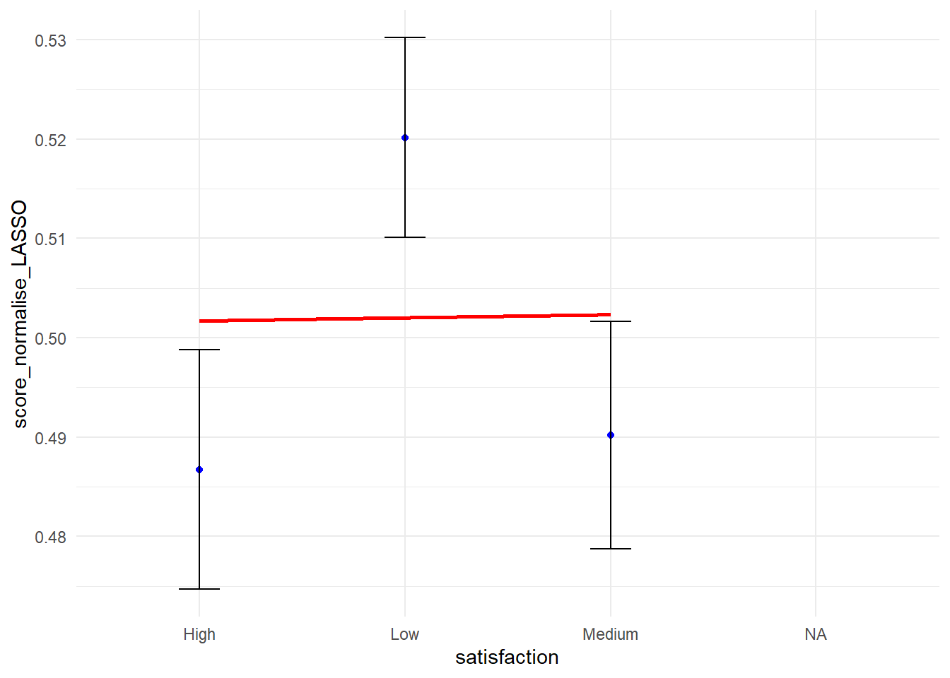
library(ggplot2)ggplot(my_data_frame, aes(x = satisfaction, y = score_normalise_LASSO)) +stat_summary(fun = mean, geom ="point", color ="blue") +stat_summary(fun.data = mean_cl_normal, geom ="errorbar", width =0.2) +geom_smooth(aes(group =1), method ="lm", se =FALSE, color ="red") +theme_minimal()
code R
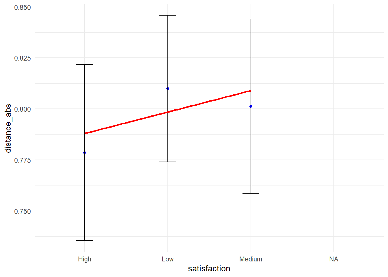
library(ggplot2)ggplot(my_data_frame, aes(x = satisfaction, y = distance_abs)) +stat_summary(fun = mean, geom ="point", color ="blue") +stat_summary(fun.data = mean_cl_normal, geom ="errorbar", width =0.2) +geom_smooth(aes(group =1), method ="lm", se =FALSE, color ="red") +theme_minimal()
code R
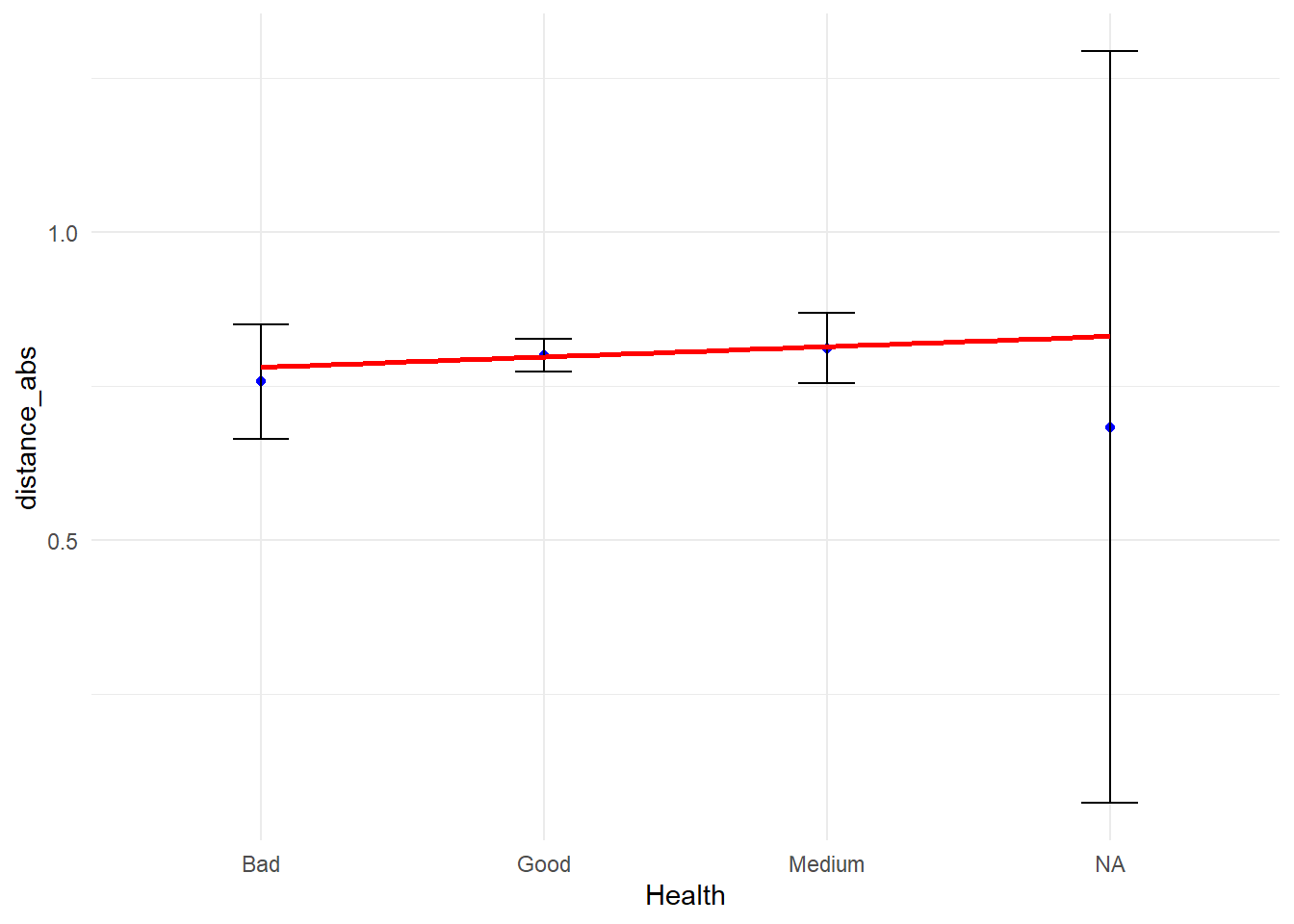
library(ggplot2)ggplot(my_data_frame, aes(x = Health, y = distance_abs)) +stat_summary(fun = mean, geom ="point", color ="blue") +stat_summary(fun.data = mean_cl_normal, geom ="errorbar", width =0.2) +geom_smooth(aes(group =1), method ="lm", se =FALSE, color ="red") +theme_minimal()
code R
library(nnet)model1 <-multinom(A15 ~ score_normalise_LASSO, data = my_data_frame)
# weights:  21 (12 variable)
initial  value 5008.772724
iter  10 value 3254.829129
iter  20 value 3133.642779
iter  30 value 3133.430501
iter  40 value 3133.386324
final  value 3133.383358
converged
code R
model2 <-multinom(A15 ~ Sex, data = my_data_frame)
# weights:  21 (12 variable)
initial  value 17968.534316
iter  10 value 13042.004757
iter  20 value 12264.214947
iter  30 value 12263.403578
iter  40 value 12263.370539
final  value 12263.370116
converged
code R
model3 <-multinom(A15 ~ score_normalise_LASSO + Sex, data = my_data_frame)
# weights:  28 (18 variable)
initial  value 5008.772724
iter  10 value 3224.638944
iter  20 value 3133.201044
iter  30 value 3131.854173
final  value 3131.795249
converged
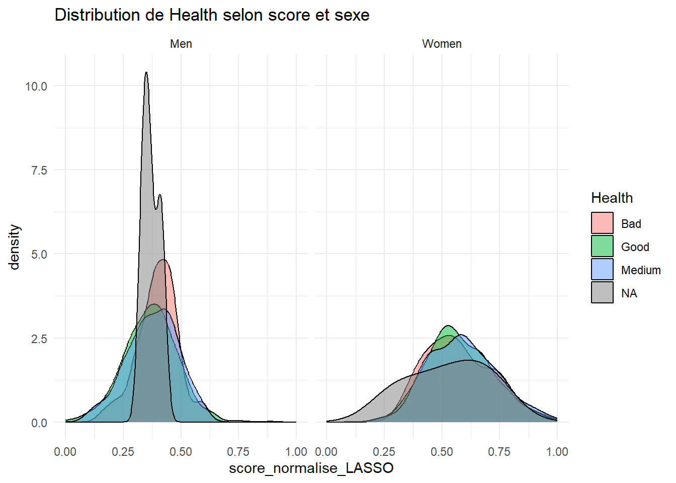
library(caret)library(vip)ggplot(my_data_frame, aes(x = score_normalise_LASSO, fill = Health)) +geom_density(alpha =0.5) +facet_wrap(~ Sex) +labs(title ="Distribution de Health selon score et sexe") +theme_minimal()