code R
############################################
# CHUNK – ACM + LASSO + Tableaux et visualisation (Dim 2 pour ACM)
############################################

library(tidyverse)
library(FactoMineR)
library(factoextra)
library(glmnet)
library(ggplot2)
library(knitr)
library(gridExtra)

# -----------------------------
# 0. Chargement des données
# -----------------------------
data <- read.csv2("pc18_quetelet_octobre2023.csv")
data$Sex <- factor(data$SEXE, levels = c(1,2), labels = c("Men","Women"))

# Renommage pratiques culturelles
my_data <- data %>%
  dplyr::rename(
    Knitting = A1001, Cards_games = A1002, Gambling = A1003,
    Cooking = A1004, DIY = A1005, Vegetable_garden = A1006,
    Ornamental_garden = A1007, Fishing_hunting = A1008,
    Collection = A1009, Vehicle_custom = A1010,
    Making_music = A1901, Diary = A1902, Writing = A1903,
    Painting = A1904, Montage = A1905, Circus = A1906,
    Pottery = A1907, Theater = A1908, Drawing = A1909,
    Dancing = A1910, Photography = A1911, Genealogy = A1912,
    Science = A1913, Video_games = B1
  )

culture_vars <- c(
  "Knitting","Cards_games","Gambling","Cooking","DIY",
  "Vegetable_garden","Ornamental_garden","Fishing_hunting",
  "Collection","Vehicle_custom","Making_music","Diary",
  "Writing","Painting","Montage","Circus","Pottery",
  "Theater","Drawing","Dancing","Photography",
  "Genealogy","Science","Video_games"
)

# Binarisation (NA = non-pratique)
my_data[culture_vars] <- lapply(my_data[culture_vars], function(x){
  x <- ifelse(x == 1, "Yes", "No")
  x[is.na(x)] <- "No"
  factor(x)
})

# -----------------------------
# 1. ACM – dimension 2 pour le genre
# -----------------------------
acm_res <- MCA(my_data[culture_vars], ncp = 5, graph = FALSE)
my_data$indice_ACM <- acm_res$ind$coord[,2]  # Dim 2
my_data$indice_ACM_norm <- (my_data$indice_ACM - min(my_data$indice_ACM)) /
                           (max(my_data$indice_ACM) - min(my_data$indice_ACM))

weights_acm <- data.frame(
  Activity = rownames(acm_res$var$coord),
  Coef_ACM = round(acm_res$var$coord[,2],3)
) %>% arrange(desc(abs(Coef_ACM)))

# -----------------------------
# 2. LASSO
# -----------------------------
X <- my_data[culture_vars] %>% mutate_all(~ ifelse(.=="Yes",1,0)) %>% as.matrix()
y <- ifelse(my_data$Sex=="Women",1,0)

set.seed(123)
cv_lasso <- cv.glmnet(X, y, family="binomial", alpha=1)
coef_lasso <- coef(cv_lasso, s="lambda.min")

lasso_weights <- data.frame(
  Activity = rownames(coef_lasso),
  Coef_LASSO = round(as.numeric(coef_lasso),3)
) %>% filter(Coef_LASSO != 0, Activity != "(Intercept)") %>%
  arrange(desc(abs(Coef_LASSO)))

my_data$score_LASSO <- as.numeric(X[, lasso_weights$Activity] %*% lasso_weights$Coef_LASSO)
my_data$score_LASSO_norm <- (my_data$score_LASSO - min(my_data$score_LASSO)) /
                            (max(my_data$score_LASSO) - min(my_data$score_LASSO))

# -----------------------------
# 3. Tableaux séparés
# -----------------------------
cat("\n### Coefficients ACM (Dim 2)\n")
### Coefficients ACM (Dim 2)code R
kable(weights_acm, caption="Coefficients ACM par activité (Dim 2)")| Activity | Coef_ACM | |
|---|---|---|
| Vegetable_garden_Yes | Vegetable_garden_Yes | 1.100 |
| Fishing_hunting_Yes | Fishing_hunting_Yes | 1.013 |
| Ornamental_garden_Yes | Ornamental_garden_Yes | 0.796 |
| DIY_No | DIY_No | -0.626 |
| Ornamental_garden_No | Ornamental_garden_No | -0.606 |
| DIY_Yes | DIY_Yes | 0.542 |
| Collection_Yes | Collection_Yes | 0.540 |
| Theater_Yes | Theater_Yes | -0.513 |
| Circus_Yes | Circus_Yes | -0.478 |
| Writing_Yes | Writing_Yes | -0.449 |
| Diary_Yes | Diary_Yes | -0.429 |
| Vegetable_garden_No | Vegetable_garden_No | -0.426 |
| Vehicle_custom_Yes | Vehicle_custom_Yes | 0.396 |
| Dancing_Yes | Dancing_Yes | -0.335 |
| Knitting_Yes | Knitting_Yes | 0.290 |
| Genealogy_Yes | Genealogy_Yes | 0.234 |
| Gambling_Yes | Gambling_Yes | 0.215 |
| Photography_Yes | Photography_Yes | 0.210 |
| Making_music_Yes | Making_music_Yes | -0.176 |
| Pottery_Yes | Pottery_Yes | 0.160 |
| Cooking_No | Cooking_No | -0.145 |
| Cooking_Yes | Cooking_Yes | 0.115 |
| Fishing_hunting_No | Fishing_hunting_No | -0.114 |
| Drawing_Yes | Drawing_Yes | -0.112 |
| Dancing_No | Dancing_No | 0.104 |
| Video_games_Yes | Video_games_Yes | -0.101 |
| Cards_games_No | Cards_games_No | -0.095 |
| Cards_games_Yes | Cards_games_Yes | 0.093 |
| Making_music_No | Making_music_No | 0.091 |
| Diary_No | Diary_No | 0.083 |
| Theater_No | Theater_No | 0.083 |
| Montage_Yes | Montage_Yes | -0.077 |
| Photography_No | Photography_No | -0.072 |
| Writing_No | Writing_No | 0.064 |
| Video_games_No | Video_games_No | 0.064 |
| Gambling_No | Gambling_No | -0.058 |
| Science_Yes | Science_Yes | 0.055 |
| Knitting_No | Knitting_No | -0.054 |
| Collection_No | Collection_No | -0.043 |
| Drawing_No | Drawing_No | 0.034 |
| Genealogy_No | Genealogy_No | -0.031 |
| Pottery_No | Pottery_No | -0.019 |
| Painting_Yes | Painting_Yes | -0.018 |
| Circus_No | Circus_No | 0.016 |
| Vehicle_custom_No | Vehicle_custom_No | -0.014 |
| Montage_No | Montage_No | 0.014 |
| Science_No | Science_No | -0.007 |
| Painting_No | Painting_No | 0.005 |
code R
cat("\n### Coefficients LASSO\n")
### Coefficients LASSOcode R
kable(lasso_weights, caption="Coefficients LASSO par activité")| Activity | Coef_LASSO |
|---|---|
| Knitting | 3.020 |
| Vehicle_custom | -1.636 |
| Dancing | 1.594 |
| Diary | 1.459 |
| Fishing_hunting | -1.432 |
| Cooking | 1.164 |
| DIY | -1.102 |
| Montage | -0.990 |
| Science | -0.799 |
| Collection | -0.678 |
| Painting | 0.541 |
| Pottery | 0.517 |
| Gambling | -0.412 |
| Photography | -0.396 |
| Vegetable_garden | -0.364 |
| Genealogy | -0.278 |
| Ornamental_garden | 0.261 |
| Cards_games | 0.167 |
| Video_games | -0.143 |
| Writing | -0.133 |
| Theater | -0.126 |
| Drawing | -0.119 |
| Making_music | -0.114 |
code R
# -----------------------------
# 4. Visualisation
# -----------------------------
p1 <- ggplot(my_data, aes(x=indice_ACM_norm, fill=Sex)) +
  geom_histogram(bins=30, alpha=0.6, position="identity", color="white") +
  scale_fill_manual(values=c("Men"="#E76F51","Women"="#3CB4C4")) +
  theme_minimal() +
  labs(x="Score ACM normalisé (Dim 2)", y="Effectifs", title="Distribution ACM par sexe")

p2 <- ggplot(my_data, aes(x=score_LASSO_norm, fill=Sex)) +
  geom_histogram(bins=30, alpha=0.6, position="identity", color="white") +
  scale_fill_manual(values=c("Men"="#E76F51","Women"="#3CB4C4")) +
  theme_minimal() +
  labs(x="Score LASSO normalisé", y="Effectifs", title="Distribution LASSO par sexe")


grid.arrange(p1, p2, ncol=1)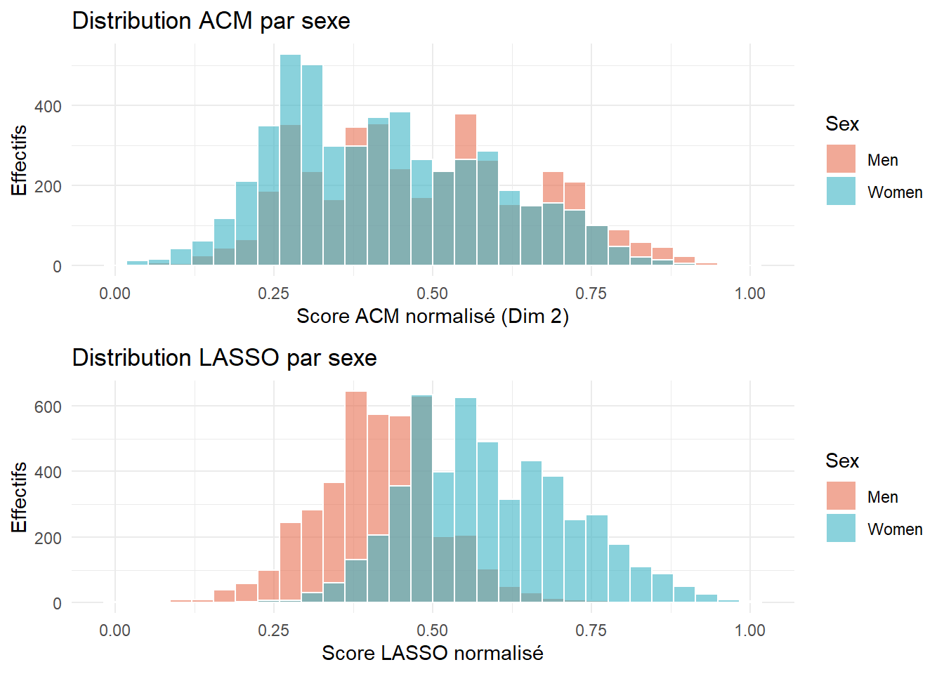
code R
# -----------------------------
# 5. Sauvegarde RDS pour Shiny
# -----------------------------
dir.create("data", showWarnings = FALSE)

saveRDS(my_data, file="data/df_model_with_scores.rds")
saveRDS(lasso_weights, file="data/coeffs_lasso.rds")
saveRDS(weights_acm, file="data/coeffs_acm.rds")
saveRDS(data.frame(
  LASSO = c(min=my_data$score_LASSO, max=my_data$score_LASSO),
  ACM   = c(min=my_data$indice_ACM, max=my_data$indice_ACM)
), file="data/bornes_scores.rds")

cat("✅ Données et coefficients sauvegardés dans 'data/'\n")
✅ Données et coefficients sauvegardés dans 'data/'code R
# -----------------------------
# 8. Robustesse des indices – par activité
# -----------------------------

# Variable cible
my_data$Sex_bin <- ifelse(my_data$Sex == "Women", 1, 0)

robustness_indices <- data.frame(
  Activity = character(),
  N = numeric(),
  Accuracy_ACM = numeric(),
  Accuracy_LASSO = numeric(),
  stringsAsFactors = FALSE
)

for (activity in culture_vars) {

  # Sous-échantillon : pratiquants
  sub_data <- my_data %>%
    filter(.data[[activity]] == "Yes")

  # Sécurité échantillon trop petit
  if (nrow(sub_data) < 30) next

  # Prédictions
  pred_acm   <- ifelse(sub_data$indice_ACM_norm >= 0.5, 1, 0)
  pred_lasso <- ifelse(sub_data$score_LASSO_norm  >= 0.5, 1, 0)

  # Accuracy
  acc_acm   <- mean(pred_acm   == sub_data$Sex_bin) * 100
  acc_lasso <- mean(pred_lasso == sub_data$Sex_bin) * 100

  # Stockage
  robustness_indices <- rbind(
    robustness_indices,
    data.frame(
      Activity = activity,
      N = nrow(sub_data),
      Accuracy_ACM = round(acc_acm, 2),
      Accuracy_LASSO = round(acc_lasso, 2)
    )
  )
}

# Tri par performance LASSO
robustness_indices <- robustness_indices %>%
  arrange(desc(Accuracy_LASSO))

# Affichage
kable(
  robustness_indices,
  caption = "Robustesse des indices ACM et LASSO – accuracy par activité (pratiquants)"
)| Activity | N | Accuracy_ACM | Accuracy_LASSO |
|---|---|---|---|
| Knitting | 1443 | 48.09 | 94.94 |
| Vehicle_custom | 324 | 47.53 | 87.04 |
| Fishing_hunting | 934 | 33.19 | 86.30 |
| Diary | 1491 | 34.00 | 84.44 |
| Dancing | 2192 | 32.30 | 84.44 |
| Pottery | 969 | 46.75 | 82.04 |
| Collection | 676 | 49.11 | 81.21 |
| Science | 1080 | 49.91 | 80.00 |
| Painting | 1970 | 42.64 | 79.75 |
| Montage | 1429 | 46.68 | 79.57 |
| Gambling | 1960 | 44.64 | 79.49 |
| DIY | 4950 | 44.38 | 79.49 |
| Cooking | 5158 | 40.31 | 79.37 |
| Vegetable_garden | 2580 | 44.65 | 79.34 |
| Ornamental_garden | 3991 | 42.77 | 79.25 |
| Photography | 2351 | 42.79 | 79.24 |
| Theater | 1283 | 39.59 | 79.03 |
| Cards_games | 4663 | 41.41 | 78.55 |
| Writing | 1156 | 40.14 | 78.37 |
| Making_music | 3142 | 42.93 | 78.07 |
| Drawing | 2149 | 44.07 | 77.90 |
| Genealogy | 1088 | 49.36 | 77.76 |
| Video_games | 3587 | 44.27 | 77.14 |
| Circus | 295 | 47.12 | 75.59 |
code R
# -----------------------------
# Variante : pratiquants / non-pratiquants
# -----------------------------

robustness_indices_full <- data.frame()

for (activity in culture_vars) {
  for (status in c("Yes", "No")) {

    sub_data <- my_data %>%
      filter(.data[[activity]] == status)

    if (nrow(sub_data) < 30) next

    pred_acm   <- ifelse(sub_data$indice_ACM_norm >= 0.5, 1, 0)
    pred_lasso <- ifelse(sub_data$score_LASSO_norm  >= 0.5, 1, 0)

    robustness_indices_full <- rbind(
      robustness_indices_full,
      data.frame(
        Activity = activity,
        Status = status,
        N = nrow(sub_data),
        Accuracy_ACM = round(mean(pred_acm == sub_data$Sex_bin) * 100, 2),
        Accuracy_LASSO = round(mean(pred_lasso == sub_data$Sex_bin) * 100, 2)
      )
    )
  }
}

kable(
  robustness_indices_full,
  caption = "Robustesse des indices ACM et LASSO selon la pratique"
)| Activity | Status | N | Accuracy_ACM | Accuracy_LASSO |
|---|---|---|---|---|
| Knitting | Yes | 1443 | 48.09 | 94.94 |
| Knitting | No | 7791 | 40.10 | 74.46 |
| Cards_games | Yes | 4663 | 41.41 | 78.55 |
| Cards_games | No | 4571 | 41.28 | 76.74 |
| Gambling | Yes | 1960 | 44.64 | 79.49 |
| Gambling | No | 7274 | 40.46 | 77.17 |
| Cooking | Yes | 5158 | 40.31 | 79.37 |
| Cooking | No | 4076 | 42.66 | 75.49 |
| DIY | Yes | 4950 | 44.38 | 79.49 |
| DIY | No | 4284 | 37.84 | 75.54 |
| Vegetable_garden | Yes | 2580 | 44.65 | 79.34 |
| Vegetable_garden | No | 6654 | 40.07 | 77.01 |
| Ornamental_garden | Yes | 3991 | 42.77 | 79.25 |
| Ornamental_garden | No | 5243 | 40.26 | 76.44 |
| Fishing_hunting | Yes | 934 | 33.19 | 86.30 |
| Fishing_hunting | No | 8300 | 42.27 | 76.69 |
| Collection | Yes | 676 | 49.11 | 81.21 |
| Collection | No | 8558 | 40.73 | 77.38 |
| Vehicle_custom | Yes | 324 | 47.53 | 87.04 |
| Vehicle_custom | No | 8910 | 41.12 | 77.32 |
| Making_music | Yes | 3142 | 42.93 | 78.07 |
| Making_music | No | 6092 | 40.53 | 77.45 |
| Diary | Yes | 1491 | 34.00 | 84.44 |
| Diary | No | 7743 | 42.76 | 76.35 |
| Writing | Yes | 1156 | 40.14 | 78.37 |
| Writing | No | 8078 | 41.52 | 77.56 |
| Painting | Yes | 1970 | 42.64 | 79.75 |
| Painting | No | 7264 | 41.00 | 77.09 |
| Montage | Yes | 1429 | 46.68 | 79.57 |
| Montage | No | 7805 | 40.37 | 77.31 |
| Circus | Yes | 295 | 47.12 | 75.59 |
| Circus | No | 8939 | 41.16 | 77.73 |
| Pottery | Yes | 969 | 46.75 | 82.04 |
| Pottery | No | 8265 | 40.71 | 77.14 |
| Theater | Yes | 1283 | 39.59 | 79.03 |
| Theater | No | 7951 | 41.63 | 77.44 |
| Drawing | Yes | 2149 | 44.07 | 77.90 |
| Drawing | No | 7085 | 40.52 | 77.59 |
| Dancing | Yes | 2192 | 32.30 | 84.44 |
| Dancing | No | 7042 | 44.16 | 75.55 |
| Photography | Yes | 2351 | 42.79 | 79.24 |
| Photography | No | 6883 | 40.85 | 77.12 |
| Genealogy | Yes | 1088 | 49.36 | 77.76 |
| Genealogy | No | 8146 | 40.28 | 77.65 |
| Science | Yes | 1080 | 49.91 | 80.00 |
| Science | No | 8154 | 40.21 | 77.35 |
| Video_games | Yes | 3587 | 44.27 | 77.14 |
| Video_games | No | 5647 | 39.49 | 77.99 |
code R
# La robustesse des indices est testée en comparant leur accuracy prédictive du genre au sein de sous-échantillons définis par chaque pratique culturelle.